Getting Started
The launch page
When you open the Escher launch page, you will see a number of options:
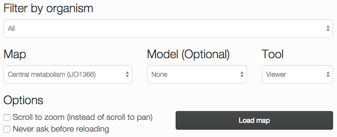
Filter by organism: Choose an organism to filter the Maps and Models.
Map: Choose a pre-built map, or start from scratch with an empty builder by choosing None.
Model: (Optional) Choose a COBRA model to load, for building reactions. You can also load your own model after you launch the tool.
Tool:
- The Viewer allows you to pan and zoom the map, and to assign data to reactions, genes, and metabolites.
- The Builder, in addition to the Viewer features, allows you to add reactions, move and rotate existing reactions, and adjust the map canvas.
Options:
- Scroll to zoom (instead of scroll to pan): Determines the effect of using the mouse’s scroll wheel over the map.
- Never ask before reloading: If this is checked, then you will not be warned before leaving the page, even if you have unsaved changes.
Choose Load map to open the Escher map in a new tab or window.
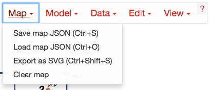
Loading and saving maps and models
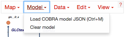
Generating COBRA model JSON files
Generating COBRA models that can be imported into Escher requires the latest beta version of COBRApy which can be found here.
Once you have COBRApy v0.3.0b1 (or later) installed, then you can generate a JSON model by following this example code.
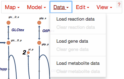
Loading reaction, gene, and metabolite data
Datasets can be loaded as CSV files or JSON files, using the Data Menu.
CSV files should have 1 header row, 1 ID column, and either 1 or 2 columns for data values. Here is an example with a single data value columns:
ID,time 0sec
glc__D_c,5.4
g6p__D_c,2.3
Which might look like this is Excel:
| ID | time 0sec |
|---|---|
| glc__D_c | 5.4 |
| g6p_c | 2.3 |
If two datasets are provided, then the Escher map will display the difference between the datasets. In the Settings menu, the Comparison setting allows you to choose between comparison functions (Fold Change, Log2(Fold Change), and Difference). With two datasets, the CSV file looks like this:
| ID | time 0sec | time 5s |
|---|---|---|
| glc__D_c | 5.4 | 10.2 |
| g6p_c | 2.3 | 8.1 |
Data can also be loaded from a JSON file. This Python code snippet provides an example of generating the proper format for single reaction data values and for reaction data comparisons:
import json

# save a single flux vector as JSON
flux_dictionary = {'glc__D_c': 5.4, 'g6p_c': 2.3}
with open('out.json', 'w') as f:
    json.dump(flux_dictionary, f)

# save a flux comparison as JSON
flux_comp = [{'glc__D_c': 5.4, 'g6p_c': 2.3}, {'glc__D_c': 10.2, 'g6p_c': 8.1}]
with open('out_comp.json', 'w') as f:
    json.dump(flux_comp, f)
Gene data and gene reaction rules
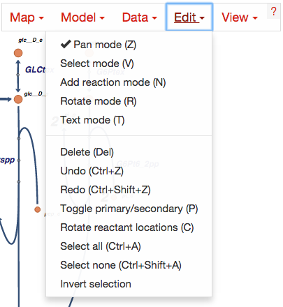
Editing and building
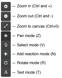
Common functions can be accessed using the buttons in the bar on the left of the screen.
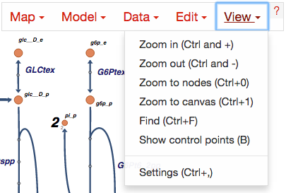
View options